Machine learning concepts. Network training and evaluation
1. Building a network model according to the problem being solved
The neural network model consists of two layers – an LSTM layer and an output Dense layer. The reason for choosing an LSTM layer is the need to process sequences of time-related data and to find data correlations. To perform these operations is needed a layer with memory, such as the LSTM layer that is capable of detecting long-term dependencies. The Dense layer limits the number of output parameters to one (corresponding to the closing price), applying an activating function to the outputs of the previous layer. A linear activation function is chosen for the Dense layer so that the neural network can predict higher values than those it was trained with. This can not be achieved with a hyperbolic tangent activation function or a logical sigmoidal activation function.
2. Setting up network hyperparameters
2.1. Batch size
Batch size is the number of examples propagated through the network. With a selected value of 100 for this hyperparameter, the algorithm divides the training data into groups of 100 records and trains the network with each of the groups. A good starting point when tuning the batch size is 32. Other common choices are 64 and 128.
2.2. Number of epochs and number of iterations
2.3. Learning rate
It is one of the most important hyperparamers. Too small or too large values for the learning rate may lead to very poor, very slow or no training. Values typically range from 0.1 to 1.10-6. 1.10-3 is a good starting point to experiment with.
2.4. Activation functions
The LSTM layer has a sigmoidal activating function used to control the LSTM gates because the sigmoidal function has output values ranging from 0 to 1. A linear activation function is selected for the Dense layer activation function.
2.5. Loss function
The mean squared error function is used for solving this regression problem. The produced error by the neural network is measured as the arithmetic mean of the sum of the differences between the predictions and the actual observations on the degree of two. The following formula gives a better explanation of the equation.

3. Network training
After creating and configuring the neural network model, the training process takes place, where the network is trained on the training data. The following graph shows the process of training the neural network. The blue line represents the correct outputs for each example, and the orange one – the predictions made by the network.

4. Network testing
The testing determines how satisfactory the predictions made by the neural network are. The network predicts data that it has not seen, and the predicted values are compared to the correct outputs. The smaller the deviations between the two values, the better predictions it makes. The following graph shows the process of testing the neural network. The blue line represents the correct outputs for each example, and the orange one – the predictions made by the network.

5. Comparing the results
After comparing the two graphs it can be easily seen that the errors on the test data are greater than those on the training. This is the expected result of the comparison. By looking at the test graph, we come to the conclusion that the results of the predictions are satisfactory. The neural network has managed to predict the trend of the cryptocurrency’s market closing price. The next thing we can do is to try other network configurations or fine tune the hyperparameters of the network.
6. Tuning the hyperparameters in order to achieve more satisfactory results
Here is a series of different combinations of hyperparametric values in order to achieve more accurate predictions. The results of the experiments are presented in the following figures. Each of the combinations is trained using the “Early stopping” method.
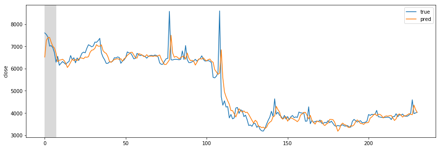
Training graph. Learning rate: 10-3, batch size: 32, number of neurons in the hidden layer: 64, loss function error: 0.0040
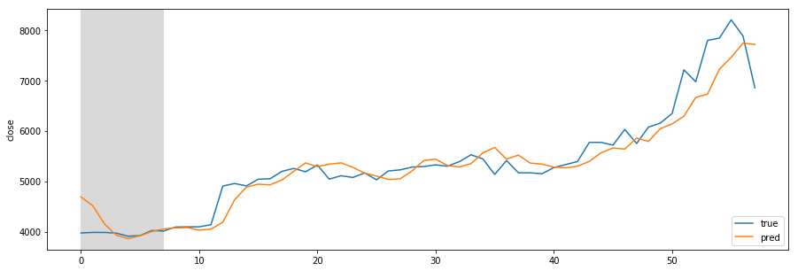
Testing graph. Learning rate: 10-3, batch size: 32, number of neurons in the hidden layer: 64, loss function error: 0.0042
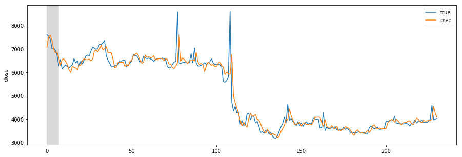
Training graph. Learning rate: 10-3, batch size: 32, number of neurons in the hidden layer: 128, loss function error: 0.0036

Testing graph. Learning rate: 10-3, batch size: 32, number of neurons in the hidden layer: 128, loss function error: 0.0038
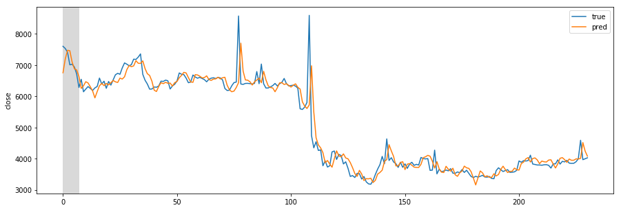
Training graph. Learning rate: 10-3, batch size: 32, number of neurons in the hidden layer: 256, loss function error: 0.0037

Testing graph. Learning rate: 10-3, batch size: 32 number of neurons in the hidden layer: 256, loss function error: 0.0037
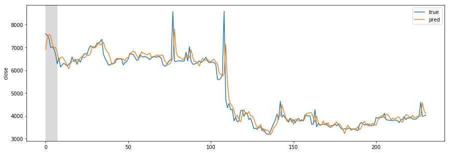
Training graph. Learning rate: 10-3, batch size: 32, number of neurons in the hidden layer: 512, loss function error: 0.0034
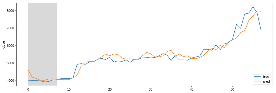
Testing graph. Learning rate: 10-3, batch size: 32 number of neurons in the hidden layer: 512, loss function error: 0.0037

Training graph Learning rate: 10-3, batch size: 64, number of neurons in the hidden layer: 512, loss function error: 0.0036
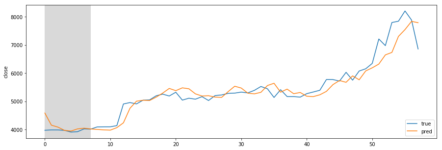
Testing graph. Learning rate: 10-3, batch size: 64, number of neurons in the hidden layer: 512, loss function error: 0.0036
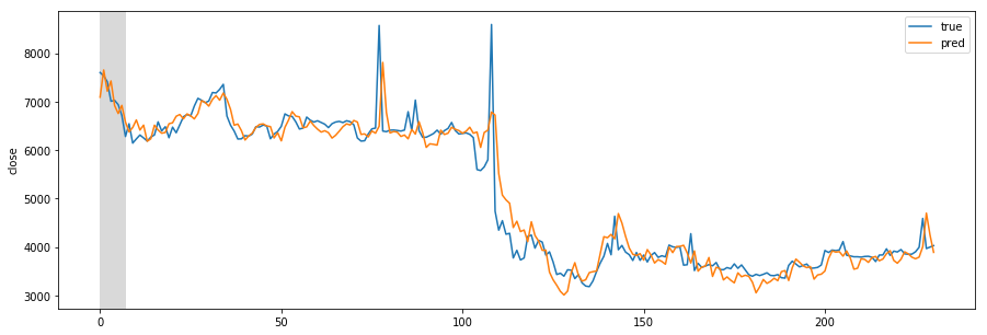
Training graph. Learning rate: 10-3, batch size: 128, number of neurons in the hidden layer: 512, loss function error: 0.0029
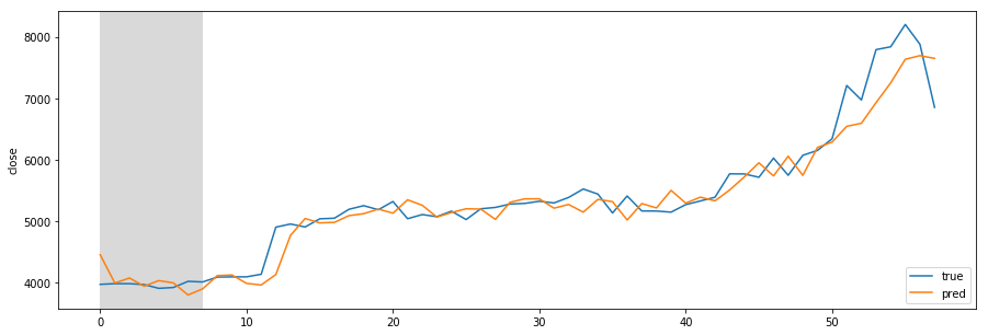
Testing graph. Learning rate: 10-3, batch size: 128, number of neurons in the hidden layer: 512, loss function error: 0.0029
- learning rate: 1.10-3
- batch size: 128
- number of neurons in the hidden layer: 512
7. Persisting the trained model. Exporting the model for further use and loading in other environments
Letzte Beiträge
Share :
Share :
Weitere Beiträge

Designing REST API architecture
The web layer is the top layer in the architecture. It is responsible for processing user queries and returning back responses to the user. These operations happen in the controllers.

Room. Reactive queries
Room has great integration with LiveData. Results from SQL queries can be easily wrapped in LiveData container. This way LiveData can be observed in the UI. When the data is changed in the database, all active observers get notified and update the corresponding views.

View in the MVVM architecture
The View component in the MVVM architecture are the UI controllers – Activities and Fragments. They should be as free as possible from any business logic. Their role is to present the data, not to transform it.

